Yield Curve, Zero Rates, and Term Structure

Introduction

Before starting my studies in Quantitative Finance I was working for a while in the banking sector and I was able to see some interesting topics other divisions were working on. The Fixed Income division, among the others, is the one that caught my attention. There was just one problem - I was able to understand very little of what they would be discussing or talking about. Some of the topics that I remember hearing a lot about were yield curve and forward rates.

The yield curve was the winner between the two when it comes to the number of times it was mentioned. Without a strong background in Finance, I knew very little about what the yield curve actually is and even less about what it tells us.

With time, I have come to gain a fairly good grasp of what it is and also what it is not, and the aim of this article is to share my knowledge with hope that someone who is in a similar situation as I was two years ago may find it useful :)

Bonds and Yield to Maturity (YTM)

To be able to understand what kind of information is contained in the yield curve, we must have a look at bonds. A bond is an instrument used to issue debt that promises a payment (or a series of payments) of fixed amounts at fixed future dates. We can differentiate between:

• Zero-Coupon (ZC) Bonds

• Coupon Bonds with fixed coupons

• Coupon Bonds with floating coupons

Note

We will have a brief look at ZC bonds and coupon bonds with fixed coupons, while the floating coupon bonds will be covered in another article.

ZC bond is the simplest possible bond, and it promises a single fixed payment at some future date which is called the maturity. The money received at maturity is called the principal of the bond and it is (usually) set to be equal to 100. You can imagine a ZC bond as a piece of paper that holds the following information:

• Issuer: The party that wrote that paper and is selling it

• Maturity date: The date at which the principal will be repaid

• Principal amount: Usually is 100

Imagine that there exists a bond that promises a payment of \(100\) exactly two years from now and that such bond is currently trading at the price of \(98\). That means that if I buy that bond now for \(98\) I will have \(100\) in two years, so I can calculate what is the return (\(r\)) of such an investment:

\[98 = \frac{100}{(1+r)^2} \Rightarrow r = \sqrt{\frac{100}{98}}-1\approx 1.015\%\]

The annualized return of such investment would be \(1.015\%\).

Now let us examine a coupon bond that promises a payment of \(100\) in exactly two years, but this time we would also receive a coupon amounting to \(5\) every 6 months (including the maturity). If such a bond is trading at \(115\) and we wanted to calculate the return of such investment we would need to determine what value of \(r\) satisfies the following equation:

\[115 = \frac{5}{(1+r)^{0.5}} + \frac{5}{(1+r)^1} + \frac{5}{(1+r)^{1.5}} + \frac{105}{(1+r)^2}\]

This is not as easy to calculate as in the example above, but there are numerical procedures that would give us the result. Luckily, this is something that you would never calculate yourself. Why? Because this is already provided by many data vendors like Bloomberg or Refinitiv. My goal here was to show conceptually how that number is calculated.

Note

If you are curious, you can use one of the many calculators available online that will calculate this for you. The one I used calculated that the return on such an investment is

\[r = 2.29\%\]

Now that we have covered how to calculate the return, we need to say what that number is. Very simply, the return \(r\) is called yield to maturity and it is a rate of return that the investor would realize if the investor were to hold the bond until maturity.

Yield Curve

Now imagine that instead of only one bond with a maturity of two years, we have a whole set of bonds with different maturities. For example, let us imagine this set of bonds (with their YTMs calculated as we did above):

Bond	Maturity (in years)	YTM
Bond A	1	2%
Bond B	2	2.35%
Bond C	3	2.5%
Bond D	5	2.56%
Bond E	10	2.6%
Bond F	20	2.65%
Bond G	30	2.67%

If we would now plot these YTMs against the maturity we would get the following result.

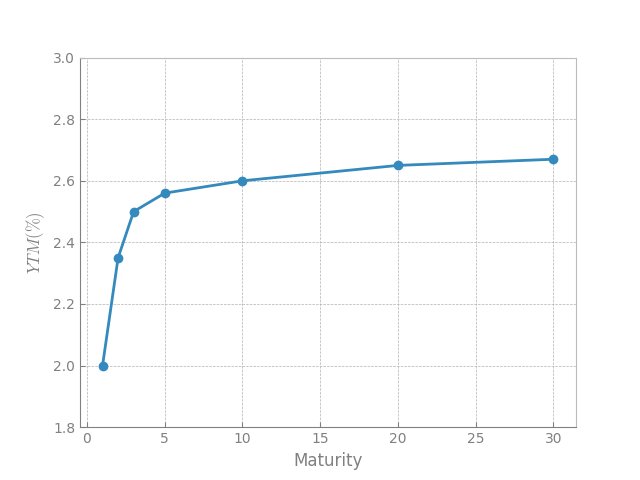
Note

The curve in the picture above is the yield curve 🙃

Zero rates

Let us quickly go back to the way that we calculated YTM for a zero coupon bond and let us take the same example - 100 principal maturing in two years currently trading at 98:

\[98 = \frac{100}{(1+r)^2}\]

Since ZC bonds have only one cash flow that cash flow has to be discounted at a unique rate of \(r\) which is determined by the current price of the bond and the principal amount that will be repaid. In this example, we calculated \(r=1.015\%\), which is

\[98 = \frac{100}{(1+1.015\%)^2}\]

We will call this bond Bond A.

Now we will introduce another ZC bond, Bond B, that matures in 1 year from now and that is currently trading at \(99\). It can easily be calculated that the YTM of this bond is \(1.010\%\):

\[99 = \frac{100}{1+1.010\%}\]

Let’s pause here for a bit and see what is the consequence of this. The main takeaway here is that cash flow that matures in 1 year has to be discounted at the rate \(r_1 = 1.010\%\) and the cash flow that matures in 2 years has to be discounted at \(r_2 = 1.015\%\). Rates \(r_1\) and \(r_2\) are called zero rates (or spot rates) for maturities of 1 year and 2 years (respectively).

Bootstrapping

Now we will introduce the third bond, Bond C, which is a coupon bond paying coupons of 10 every year and matures 3 years from now. Such a bond is currently trading at 120 and its YTM is \(2.94\%\). This means that the following equation holds:

\[120 = \frac{10}{1+2.94\%} + \frac{10}{(1+2.94\%)^2} + \frac{110}{(1+2.94\%)^{3}}\]

Another way to look at it is that we have discounted the future payments at a rate equal to YTM. In other words, if all future cash flows, no matter when they come would be discounted at the same rate (YTM) then the sum of discounted cash flows is equal to the current price of the bond.

For this reason, I avoided using the wording “discounting” above. The way we calculate YTM with coupon bonds can easily be confused with discounting, but the problem is that (normally) the cash flows with different maturities will have different discount rates \(r_i\) applied to them. Look at the first element of the sum, i.e. \(\frac{10}{1+2.94\%}\), here we are discounting the cash flow maturing in 1 year at the rate equal to \(2.94\%\), while at the same time with the Bond B we are discounting the cash flow maturing in 1 year with a discount rate of \(1.010\%\).

This seems odd, if we are talking about the same issuer we should be discounting the cash flows maturing at the same time with the same discount rate, i.e. with their respective Zero rates. With ZC bonds that is obvious, because YTM is the same as the zero rate for that maturity, so let us start with that and rewrite the equation for our Bond C:

\[120 = \frac{10}{1+1.010\%} + \frac{10}{(1+1.015\%)^2} + \frac{110}{(1+r_3)^{3}}\]

Since we do not have available a ZC bond with a maturity of 3 years, we cannot directly determine the zero rate for that maturity, but we can calculate it from the equation above:

\[ r_3 = \sqrt[3]{\frac{110}{120 -\frac{10}{1+1.010\%} - \frac{10}{(1+1.015\%)^2}}} - 1 = 3.125\%\]

And with this, we have managed to calculate the zero rates (\(r_i\)) for maturities \([1,2,3]\). Now if we would add a Bond D, which matures in 4 years from now, we could calculate the zero rate \(r_4\), and so on with higher maturities.

Important

This process of obtaining zero rates is called bootstrapping

Faster way to obtain zero rates

Let us list again the equations for our bonds B, A, and C:

\[\begin{split} \begin{split} 99 &= \frac{100}{1+r_1} \\ 98 &= \frac{100}{(1+r_2)^2} \\ 120 &= \frac{10}{1+r_1} + \frac{10}{(1+r_2)^2} + \frac{110}{(1+r_3)^{3}} \end{split} \end{split}\]

This is a system of equations and whenever we have a system of equations we can use matrix notation to write it down:

\[\begin{split} \begin{bmatrix} 100 & 0 & 0\\ 0 & 100 & 0\\ 10 & 10 & 110\\ \end{bmatrix} \cdot \begin{bmatrix} z_1\\ z_2\\ z_3 \end{bmatrix} = \begin{bmatrix} 99 \\ 98 \\ 120 \end{bmatrix} \end{split}\]

\[\begin{split}M\cdot \begin{bmatrix} z_1\\ z_2\\ z_3 \end{bmatrix} = \begin{bmatrix} 99 \\ 98 \\ 120 \end{bmatrix}\end{split}\]

where we set

\[\begin{split} \begin{split} z_1 &= \frac{1}{1+r_1}\\ z_2 &= \frac{1}{(1+r_2)^2}\\ z_3 &= \frac{1}{(1+r_3)^3} \end{split} \end{split}\]

This system of equations will have a unique solution if the rank of the matrix \(M\) is full (in this case 3). Then the inverse of the matrix exists and we can find solutions for all \(z_i\) as follows:

\[\begin{split}\begin{bmatrix} z_1\\ z_2\\ z_3 \end{bmatrix} = M^{-1}\cdot\begin{bmatrix} 99 \\ 98 \\ 120 \end{bmatrix}\end{split}\]

If we find the inverse of the matrix we get the following result:

\[\begin{split}\begin{bmatrix} z_1\\ z_2\\ z_3 \end{bmatrix} = \begin{bmatrix} \frac{1}{100} & 0 & 0\\ 0 & \frac{1}{100} & 0\\ -\frac{1}{1100} & -\frac{1}{1100} & \frac{1}{110}\\ \end{bmatrix} \cdot\begin{bmatrix} 99 \\ 98 \\ 120 \end{bmatrix} = \begin{bmatrix} 0.99 \\ 0.98 \\ \frac{1003}{1100} \end{bmatrix}\end{split}\]

This will give us the same results that we obtained with bootstrapping above:

\[\begin{split} \begin{split} r_1 &= \frac{1}{z_1} - 1 = 1.010\%\\ r_2 &= \sqrt{\frac{1}{z_2}} - 1 = 1.015\%\\ r_3 &= \sqrt[3]{\frac{1}{z_3}} - 1 = 3.125\% \end{split} \end{split}\]

Term Structure

The last thing we have to talk about is the term structure and how it is different from the yield curve. The good news is that now we basically have all the ingredients to tackle this.

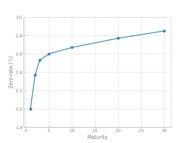
The term structure is the curve we get when we plot zero rates that we calculated against the maturity. If we plot a term structure we get a representation similar to that of the yield curve:

This is maybe one of the reasons why the term structure of interest rates is confused with the yield curve. They are two different things that look similar, and to see exactly how similar we best plot them together:

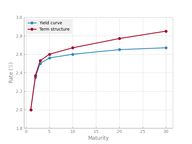
Typically we would observe such a relation between the two, i.e. the term structure is a bit above the yield curve.

Note

Please note that the numbers plotted here are purely for demonstrational purposes and do not come from any concrete example.

Summing it up

The yield curve shows us the relationship between the Yield to Maturity (YTM) and the maturity of the bond, for the bonds coming from the same issuer. YTM is the return that the investor would lock in if he/she would hold the bond until maturity.

Term structure, on the other hand, shows us the relationship between the zero rates and the maturity (of the cash flows from the certain issuer). In other words, it tells us the rate at which we need to discount the cash flows maturing at a specified time in the future, in order to calculate its present value.